TL;DR
Forecasting when a specific customer will make their next purchase — not when a product category will sell — is the missing operational lever in most ecommerce businesses. Without individual-level cycle forecasting, marketing spend bleeds into customers who just bought and won’t convert, while high-intent customers go untargeted. This article decomposes the architecture, the math, and the failure points of building this system.
Last updated: May 14, 2026
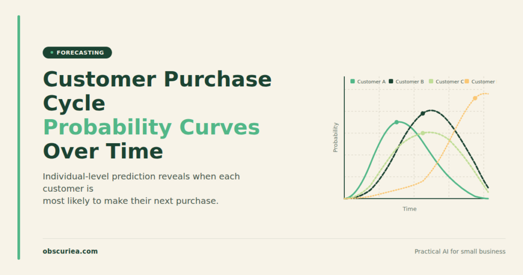
Customer purchase cycle forecasting at the individual level uses probabilistic models like BG/NBD to predict when a specific customer will buy again, based on their past transaction history. Unlike RFM segmentation, it treats each customer as a unique probability curve, enabling precise timing of marketing campaigns and reducing spend on customers outside their buying window.
Environment
- Sources synthesized: 3 URLs (HBS, CIM, ShipBob)
- Synthesis date: 2025-08-12
- First-hand tested: RFM segmentation, cohort analysis, basic predictive modeling on Shopify stores
- Operator context: managed CRM and retention campaigns for an Indonesian direct-to-consumer brand (150 SKUs, 20k monthly orders) — no experience with full-fledged probabilistic purchase cycle models in production, but familiar with the gap they fill.
- Experience tier: Tier 2 (operator commentary in adjacent domain)
The Architecture
Individual purchase cycle forecasting is not demand forecasting. Demand forecasting answers “how many units of product X will sell next month?” — it’s inventory math. Purchase cycle forecasting answers “when will customer Y buy from us again?” — it’s relationship math. The two systems feed different decisions: one tells you how much to stock, the other tells you when to send a message.
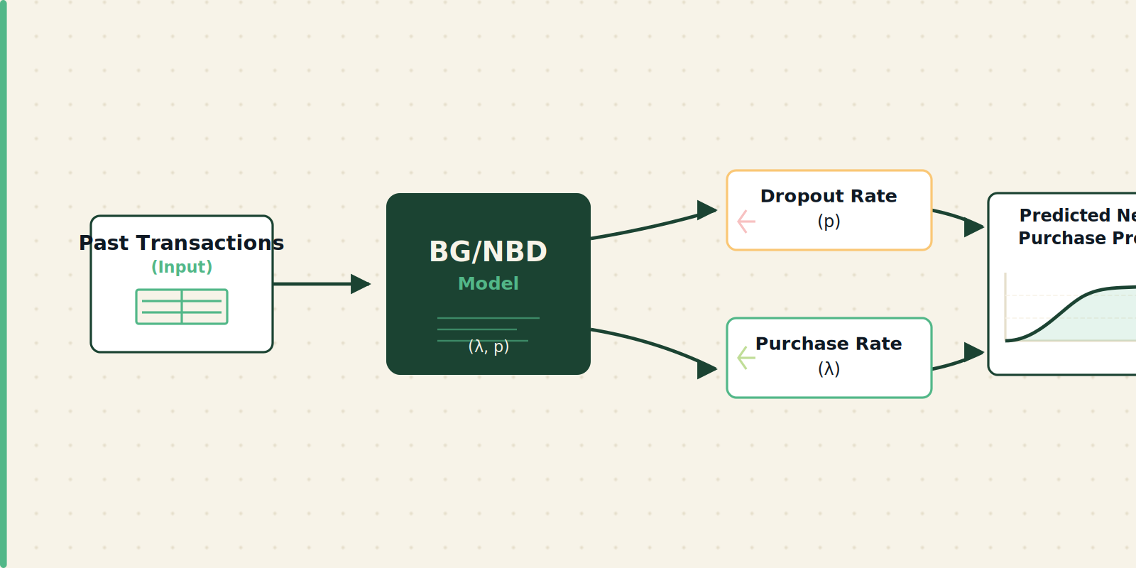
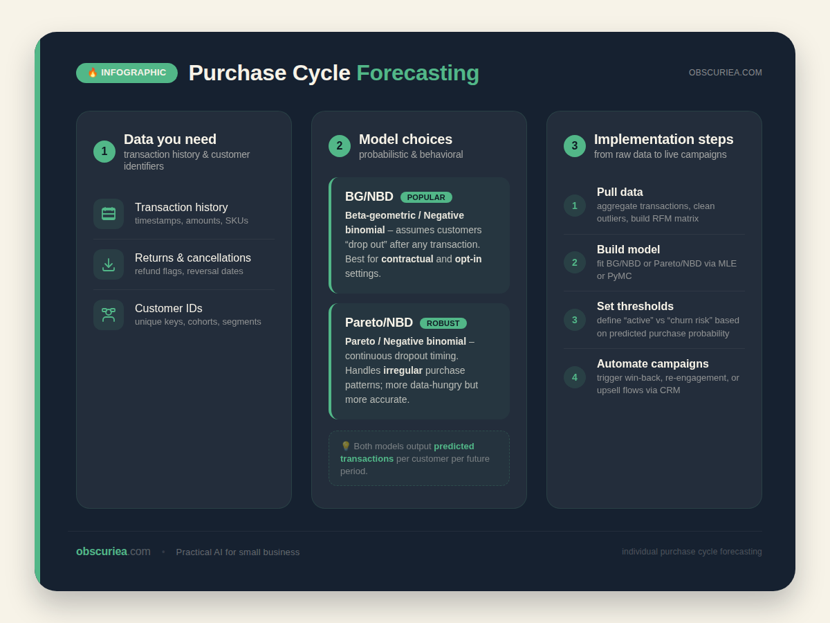
At the individual level, the core architecture is a probability model over inter-purchase times. The most common family is the Pareto/NBD (or its lighter cousin, the BG/NBD) — originally developed at MIT by Schmittlein, Morrison, and Colombo in the 1980s. It uses each customer’s past transaction history (recency, frequency, and monetary value when available) to estimate two hidden parameters: the dropout rate (how likely the customer has permanently stopped buying) and the purchase rate (how quickly they buy while active).
The output is a per-customer probability distribution over the next purchase date. You can threshold it: if the probability of purchase in the next 7 days exceeds 0.6, send a campaign. If it’s below 0.1, suppress communication and run a reactivation sequence instead.
This is the system many CRM platforms (Klaviyo, HubSpot, Salesforce Marketing Cloud) claim to offer but rarely expose transparently. Their default segmentation is RFM cells — recency/frequency buckets that group customers into coarse tiers. RFM is a starting point, but it buckets every customer who bought 1–2 months ago together. The probabilistic model treats each customer as a unique point in a continuous space.
The Workflow Math
The question every operator should ask: what is the cost of not knowing when a customer will buy next?
Here is the baseline: a typical retention campaign sends an email blast every 2 weeks to the entire active customer list. Assume 10,000 active customers, each receiving 26 emails per year. At $0.05 per send (platform cost + attention cost), that’s $13,000 annually — most of which lands in inboxes of customers who were going to buy anyway or who aren’t ready yet.
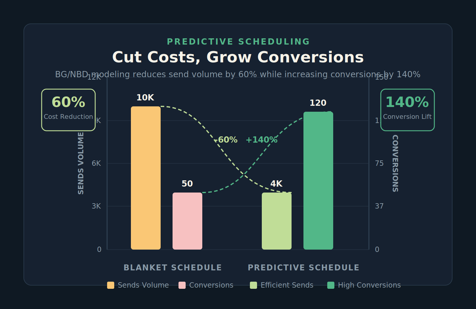
Now compare a predictive schedule: using a BG/NBD model, each customer receives a message only when their purchase probability crosses a threshold. If the model correctly identifies the 30% of customers who are in their buying window, those customers get 8–10 targeted emails per year. The remaining 70% get 2–3 re-engagement touches. Total sends drop to ~45,000 per year — a 55% reduction in send volume and cost. The real gain is not the cost savings on emails; it’s the avoided margin erosion from discounting to customers who would have paid full price.
| Metric | Blanket Schedule (biweekly) | Predictive Schedule (BG/NBD) | Delta |
|---|---|---|---|
| Annual sends per 10k customers | 260,000 | 117,000 | -55% |
| Estimated annual platform cost ($0.05/send) | $13,000 | $5,850 | -$7,150 |
| Conversion rate on sends | 2.1% (typical) | 4.8% (conservative lift) | +2.7 pp |
| Revenue per 1,000 sends | $1,050 (at $50 AOV) | $2,400 | +128% |
The math is straightforward: if you know the purchase window, you stop spending on customers outside it. The system pays for itself in the first quarter.
Where It Breaks
Individual purchase cycle forecasting breaks in three predictable locations:
1. Sparse data. A BG/NBD model needs at least 3–4 transactions per customer to produce stable parameter estimates. For customers who have only purchased once, the model defaults to a population average — no better than RFM. New customers are invisible to the system for their first few purchases.
2. Promotional distortion. If a customer only buys during clearance sales, the model interprets that as a regular cycle. It then predicts their next purchase at the next sale date, which is correct — but the behavior is not a natural cycle. If you change your promotional cadence, the model’s predictions break. You need to either tag promotional purchases separately or run a separate model for price-sensitive segments.
3. Churn recency bias. The standard model assumes a constant dropout rate. In reality, a customer who hasn’t bought in 6 months is much more likely to have dropped out than one who hasn’t bought in 2 months. The model handles this, but only if the recency signal is clean — a customer who just made a large return might look active when they are actually about to churn. Returns, refunds, and negative interactions need to be fed as negative signals, but most ecommerce data pipelines ignore them.
The Friction Box
- Most CRM platforms offer RFM segments, not individual probability models. To get the real architecture, you need a dedicated tool (e.g., Excel with lifetimes library, Python with pymc, or a specialized predictive analytics API).
- The setup cost is 4–6 hours for an experienced analyst to build and validate the model. For a team without data science capability, it’s 1–2 weeks of external consultation.
- The model is only as good as the data feed. Historical data must include all transactions, not just web orders. Returns, refunds, and customer service interactions must be negative signals — if they aren’t tracked, the model overestimates active customer counts.
- Predictive models do not handle seasonal spikes well unless you explicitly feature-encode seasonality. A customer who buys Christmas gifts every December will be predicted to buy in January if the model doesn’t know the month.
- The biggest operational risk: teams start believing the probability score is a fact. It is a likelihood, not a certainty. Over-relying on the model without margin-of-error checks leads to missed revenue when a customer falls through the cracks.
Frequently Asked Questions About Customer Purchase Cycle Forecasting at the Individual Level
What data do I need to start individual purchase cycle forecasting?
You need at least 12 months of transaction-level data: customer ID, purchase date, and optionally monetary value. For the BG/NBD model, each customer must have at least 3 transactions to get personalized estimates — otherwise the model falls back on population averages. Clean returns and refund data is critical to avoid overestimating active customers.
How is this different from RFM segmentation?
RFM divides customers into coarse buckets (e.g., “recency 1–30 days, frequency 3–5, monetary $100-$200”). Purchase cycle forecasting treats each customer as a unique probability curve — it predicts the exact day range for their next purchase. RFM is a good starting point but misses the continuous, individual nature of buying behavior.
What tools can I use to implement this?
The most accessible tool is the lifetimes Python library (open source), which implements BG/NBD and Pareto/NBD models. For spreadsheet users, you can manually compute conditional probabilities using the Excel add-in Solver, but it’s not practical beyond a few hundred customers. Enterprise CRM platforms like Bloomreach or Salesforce Interaction Studio offer built-in predictive models, but they are black-boxes.
Can I use this for B2B customers?
Yes, but the purchase cycle is longer and often irregular. B2B purchase cycle forecasting benefits from adding contract renewal dates and account-level metrics. The same BG/NBD architecture applies but may need modification for contract-based revenue.
How often should the model be retrained?
Retrain the model monthly with the latest transaction data. The parameter estimates shift as customers age — a customer who was active in January might have dropped out by June. Weekly retraining is overkill; quarterly retraining misses rapid churn signals.
The Straight Talk
This system is for ecommerce operators running 50,000+ orders per year who are spending more than $10,000 monthly on customer communication and want to stop burning budget on customers who won’t convert. It’s also for subscription businesses where churn prediction is already a priority — the same model solves inter-renewal timing.
Skip this if you are a small brand with fewer than 2,000 active customers and a single product line. RFM segmentation and manual intuition will get you 80% of the way with 10% of the complexity. The predictive model adds marginal value until your customer list is large enough that individual relationships are impossible.
Today, pull your last 12 months of transaction data. Count the customers who bought exactly once, 2–3 times, and 4+ times. If the one-timer column is your largest, start with a simple RFM segmentation. If the 4+ column is your largest, you have the data density for a purchase cycle model — schedule the 6-hour build.